// Two lanes with no lane changing; a loop at x0 averages the speeds of the cars that cross it,
// and a drone averages the speeds of all cars in view at each instant.
showdown = {
  const Lr = 360, x0 = 180, lanes = [{v: 30, s: 60}, {v: 15, s: 40}];
  const cars = [];
  lanes.forEach((ln, li) => { for (let x = 0; x < Lr; x += ln.s) cars.push({x, lane: li, v: ln.v}); });
  const dt = 1 / 60;
  let t = 0, loopN = 0, loopSum = 0, droneSum = 0, droneN = 0;
  const flash = [0, 0];
  while (true) {
    for (const c of cars) {
      const xn = c.x + c.v * dt;
      if (c.x < x0 && xn >= x0) { loopN++; loopSum += c.v; flash[c.lane] = 10; }
      c.x = xn >= Lr ? xn - Lr : xn;
    }
    droneSum += cars.reduce((s, c) => s + c.v, 0) / cars.length; droneN++;
    flash[0] = Math.max(0, flash[0] - 1); flash[1] = Math.max(0, flash[1] - 1);
    t += dt;
    yield {cars: cars.map(c => ({...c})), t, Lr, x0, flash: [...flash], loopN,
           loop: loopN ? loopSum / loopN : NaN, drone: droneSum / droneN};
  }
}2 · What Do Sensors Really Measure?
The same traffic, two different speeds · Edie’s definitions · why your phone and the road disagree
Part 1 · How we watch traffic
Two ways to watch a road
Every traffic dataset starts with a sensor, and every sensor watches the road in its own way. Meet the two we compare today.
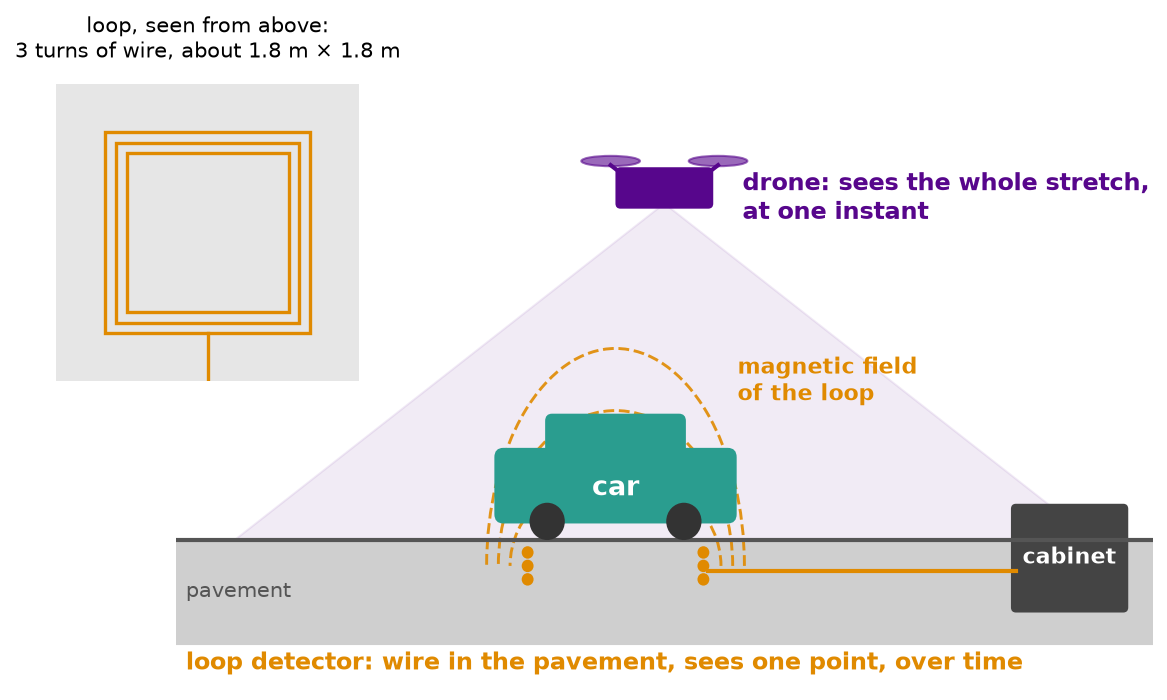
- The loop detector is a few turns of wire laid in a square cut in the pavement, about 1.8 m on a side, and wired to a cabinet by the road.
- Why a loop? Current flowing around a loop of wire makes a magnetic field above the lane: the loop is an inductor. When a car’s metal body enters that field, the loop’s inductance drops, and the electronics in the cabinet register a vehicle.
- So a loop sees one point on the road, over time: every car that crosses it.
- The drone films the road from above. It sees the whole stretch, at one instant: every car on it.
How a loop detector works
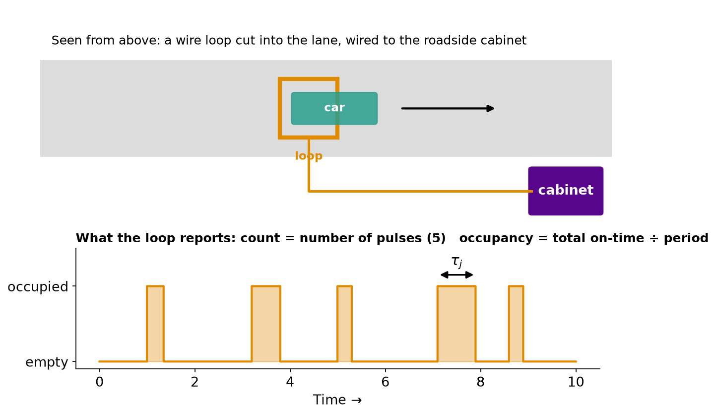
A closer look at the loop: how a coil of wire becomes counts and occupancy.
- A coil of wire in the pavement, wired to a roadside cabinet.
- A vehicle’s metal body lowers the loop’s inductance: the loop is occupied.
- Raw output: on/off presence. Every 20–30 s it becomes a count and an occupancy (share of time on).
- A single loop cannot measure speed; it is estimated (next slide).
- A dual loop, two loops a few metres apart, measures speed directly.
Classifying traffic sensors
By where they sit
- In the pavement (intrusive): loops, magnetometers, tubes, weigh-in-motion. Accurate, but the road must be closed to install or repair them.
- Above or beside the road (non-intrusive): radar, video, LiDAR, infrared, acoustic. Installed on poles and gantries, without touching the pavement.
- In the vehicle: phones, fleet GPS, connected vehicles.
- In the air: aerial photographs from aircraft, and drones.
By what they see
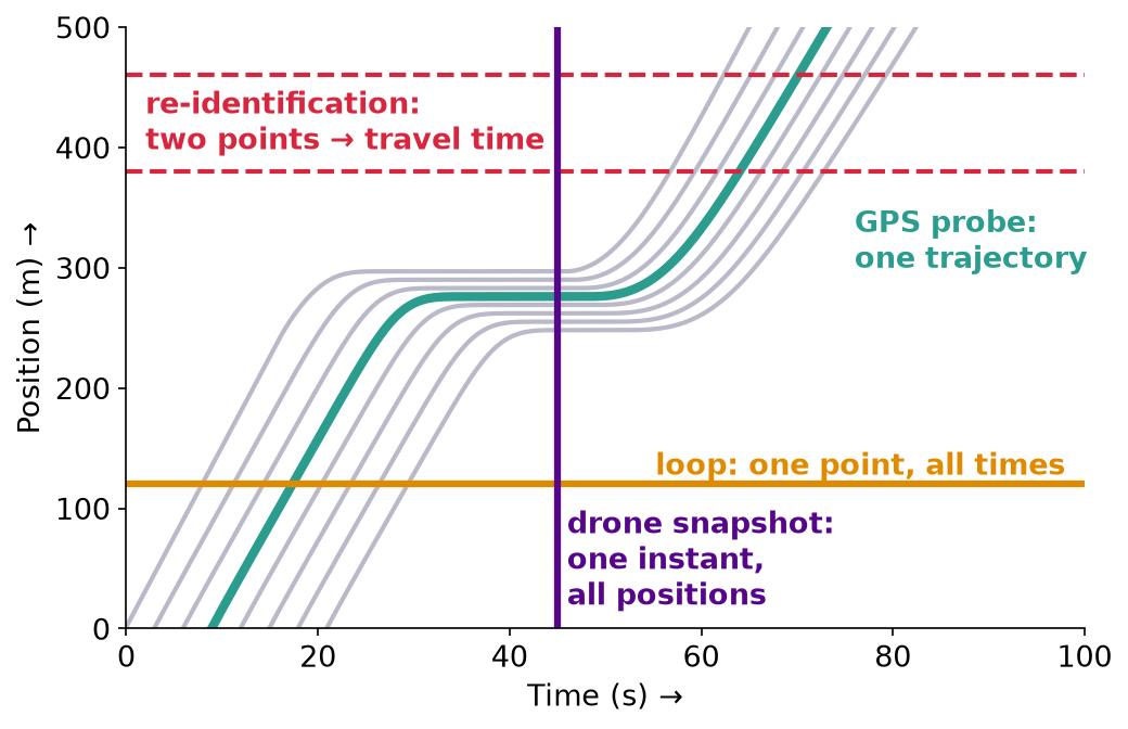
- A point: counts, occupancy, spot speeds.
- Two points: the same vehicle recognised twice, giving travel time.
- An area: every vehicle on a stretch, at an instant.
- A moving vehicle: one trajectory, or pieces of it.
A catalogue of traffic sensors
| Sensor | How it works | Data | Pros | Cons |
|---|---|---|---|---|
| Inductive loop | wire coil in the pavement; a vehicle’s metal lowers its inductance | count, occupancy; speed with two loops | mature, cheap to run, accurate counts | pavement must be cut; lane closures to repair; one loop cannot measure speed |
| Magnetometer | small puck senses the vehicle’s disturbance of Earth’s magnetic field | count, occupancy, some speed | quick to install in a small hole; often wireless | battery life; less reliable vehicle classes |
| Pneumatic tube | rubber tube across the road; each axle sends an air pulse | axle counts, vehicle class, speed with two tubes | cheap and portable, ideal for temporary counts | wears out; poor in slow or stop-and-go traffic; risky to install |
| Piezoelectric / weigh-in-motion | sensors in the pavement measure the force of each axle | axle weights, vehicle class, speed | the only way to weigh trucks at speed | expensive; needs careful calibration; pavement must be cut |
| Sensor | How it works | Data | Pros | Cons |
|---|---|---|---|---|
| Microwave radar | Doppler: frequency shift from moving vehicles. FMCW side-fire: ranges vehicles across the lanes | speed (Doppler); count, occupancy and speed by lane (FMCW) | all weather; one unit covers many lanes | Doppler cannot see stopped vehicles; tall trucks hide cars behind them |
| Video detection | cameras with image processing, now often deep learning | count, speed, class, queue length, incidents | rich information; one camera, many uses | glare, darkness, rain and snow; occlusion; privacy |
| LiDAR | laser pulses measure distance to every point in view | precise vehicle position, shape and class | very accurate 3-D picture | costly; affected by heavy rain and fog |
| Infrared | active: reflected infrared beam; passive: the vehicle’s heat | presence, count, speed | works day and night | sensitive to weather |
| Acoustic | microphone array hears the noise of passing vehicles | presence, count, speed | passive and cheap | less accurate; affected by background noise |
| Sensor | How it works | Data | Pros | Cons |
|---|---|---|---|---|
| Bluetooth / Wi-Fi readers | record anonymised device IDs at two sites and match them | travel time between the sites | cheap; easy to deploy | only a few percent of vehicles are matched; phones now randomise their IDs; privacy |
| Toll-tag readers | read electronic toll tags (for example E-ZPass) at two sites | travel time | very high match rates where tags are common | only tagged vehicles; needs reader infrastructure |
| Licence-plate cameras | read plates at two sites and match them | travel time, origin–destination patterns | nearly every vehicle can be matched | privacy and legal limits; misreads; cost |
| Sensor | How it works | Data | Pros | Cons |
|---|---|---|---|---|
| GPS probes | phones and fleet vehicles report their positions | speeds and travel times on most roads | wide coverage with no roadside hardware | sample bias and low penetration on minor roads; data licences; privacy |
| Connected vehicles | vehicles broadcast position, speed, acceleration and braking several times a second | detailed vehicle trajectories and driving behaviour | rich, high-frequency data | few equipped vehicles so far; standards and security |
| Drones | a camera films the road from above, then vehicles are tracked | full trajectories of every vehicle in view | the whole time-space diagram | short flights; regulations and weather; heavy processing |
| Aerial photographs | a camera on an aircraft photographs the road from straight above | every vehicle in view: density, and speeds from two photos a few seconds apart | a whole stretch at one instant; a classic, simple method | one moment only; flights cost money; weather and daylight |
| Floating car | a test vehicle drives with the traffic and records its trip | travel time, delay, stops | simple and direct | one vehicle’s experience; labour-intensive |
Seeing from above: aerial photos and drones
From an aircraft
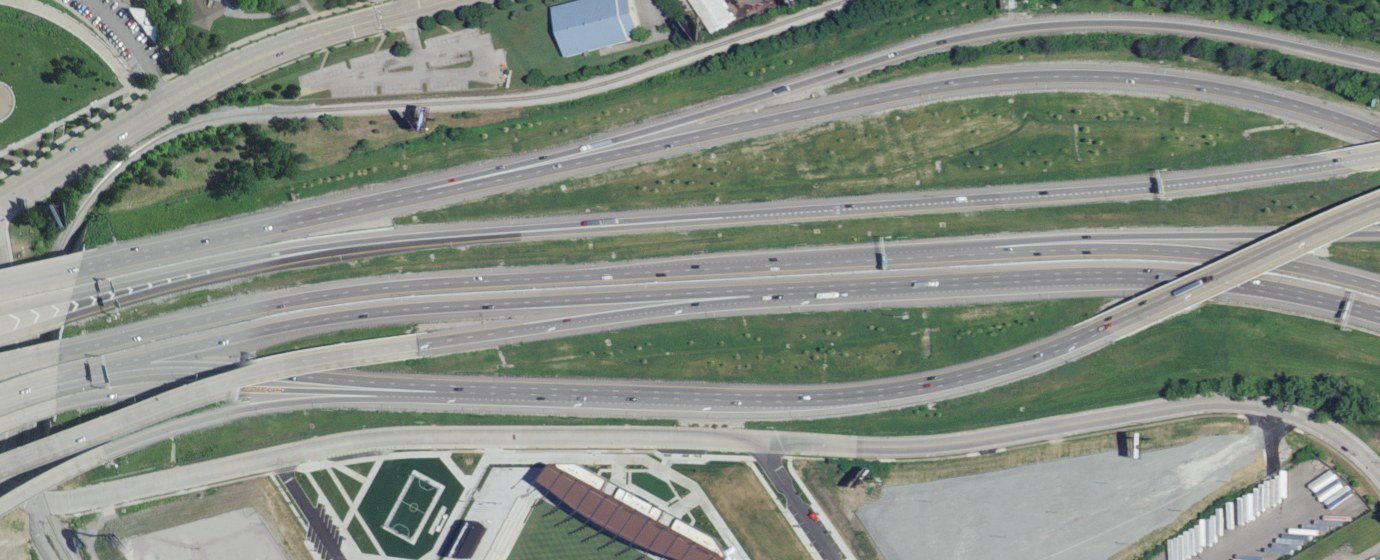
Interstate 64 in Louisville, Kentucky. Every car and truck can be counted. One photo gives the density on each lane directly; two photos a few seconds apart give every vehicle’s speed, and so the space-mean speed. Photo: NOAA (public domain).
From a drone
Downtown Athens, filmed by one of ten drones hovering over the city in the pNEUMA experiment (EPFL, 2018). Like an aerial photo, a drone sees every vehicle at once, but it keeps watching: from the video, every trajectory can be recovered. Video: pNEUMA Vision dataset, Kim, Anagnostopoulos, Barmpounakis and Geroliminis (EPFL), CC BY 4.0.
Part 2 · One road, two answers
The puzzle
A loop detector is buried in the road. A drone hovers overhead. Both watch exactly the same cars, and both report the average speed. They will not agree, and neither of them is broken.
Before you watch: predict
Which sensor will report the higher average speed: the loop in the road, or the drone in the sky? Or will they agree? Make a guess before you go on.
The sensor showdown
Two lanes: fast cars spaced out in the top lane, slow cars bunched together in the bottom lane. The orange bar is the loop detector; it flashes each time a car crosses it. The dashed frame is what the drone sees.
{
  const narrow = plotW < 640, W = narrow ? plotW : 720, left = 20, right = W - 20, sc = (right - left) / showdown.Lr;
  const laneY = [52, 92], H = 28;
  const colors = ["#2a9d8f", "#e76f51"];
  return htl.svg`<svg width="100%" viewBox="0 0 ${W} ${narrow ? 184 : 150}" role="img" aria-label="Two lanes of cars passing a loop detector under a drone">
    <rect x=${left - 8} y="22" width=${right - left + 16} height="112" fill="none" stroke=${accent} stroke-width="2" stroke-dasharray="7 5" rx="6"/>
    <text x=${left} y="16" font-size="13" fill=${accent} font-weight="bold">${narrow ? "Drone's view: whole road, one instant" : "Drone's view: the whole road, at one instant"}</text>
    ${laneY.map(y => htl.svg`<rect x=${left} y=${y - H / 2} width=${right - left} height=${H} fill="#8882"/>`)}
    ${laneY.map((y, li) => htl.svg`<rect x=${left + showdown.x0 * sc - 4} y=${y - H / 2} width="8" height=${H}
        fill=${showdown.flash[li] ? "#ff9f1c" : "#ff9f1c55"} />`)}
    ${showdown.cars.map(c => htl.svg`<rect x=${left + c.x * sc} y=${laneY[c.lane] - 8} width=${Math.max(4, 4.5 * sc)} height="16" rx="3" fill=${colors[c.lane]} />`)}
    <text x=${left + showdown.x0 * sc} y="146" font-size="12" text-anchor="middle" fill="#c77700" font-weight="bold">▲ loop detector</text>
    ${narrow
      ? htl.svg`<text x=${left} y="166" font-size="11" fill="gray">top: 108 km/h, 60 m apart</text>
               <text x=${left} y="180" font-size="11" fill="gray">bottom: 54 km/h, 40 m apart</text>`
      : htl.svg`<text x=${right} y="16" font-size="11" text-anchor="end" fill="gray">top: 108 km/h, 60 m apart · bottom: 54 km/h, 40 m apart</text>`}
  </svg>`;
}md`<div class="grid">
<div class="g-col-12 g-col-md-6 card-lite"><b>Loop detector</b> (one point, over time)<br>
<span style="font-size:2rem;font-weight:800;color:#c77700">${showdown.loopN ? (showdown.loop * 3.6).toFixed(0) + " km/h" : "waiting…"}</span><br>
<small>${showdown.loopN} cars counted so far</small></div>
<div class="g-col-12 g-col-md-6 card-lite"><b>Drone</b> (the whole road, at an instant)<br>
<span style="font-size:2rem;font-weight:800;color:${accent}">${(showdown.drone * 3.6).toFixed(0)} km/h</span><br>
<small>average of every car in view</small></div>
</div>`What just happened?
- The loop settles near 85 km/h. The drone reports 76 km/h. Same cars, same moment, a 9 km/h disagreement.
- The loop counts fast cars more often, because fast cars pass it more often.
- The drone counts slow cars more often, because slow cars spend longer on the road and bunch up.
- Neither sensor is wrong. They answer different questions, and a traffic engineer must know which question the data answered.
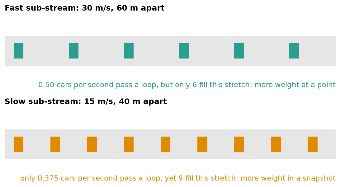
| Watching… | Like | Average speed |
|---|---|---|
| one point, over a period of time | loop detectors, radar guns, cameras | time-mean speed \(\bar v_t\) |
| a stretch of road, at one instant | drones, aerial photos | space-mean speed \(\bar v_s\) |
You drive 30 km to work at 30 km/h, and drive home at 60 km/h. What was your average speed?
Not 45 km/h. The trip took 1 h there and 0.5 h back: 60 km in 1.5 h is 40 km/h. You spent more time driving slowly, so the slow leg counts for more. That is exactly the drone’s point of view.
Build your own road
Two lanes, with no lane changing. Set each lane’s speed and spacing, and see what each sensor reports.
viewof vA = Inputs.range([5, 40], {value: 30, step: 1, label: "Lane A speed (m/s)"})
viewof sA = Inputs.range([10, 120], {value: 60, step: 5, label: "Lane A spacing (m)"})
viewof vB = Inputs.range([5, 40], {value: 15, step: 1, label: "Lane B speed (m/s)"})
viewof sB = Inputs.range([10, 120], {value: 40, step: 5, label: "Lane B spacing (m)"})
lanes = {
const qA = vA / sA, qB = vB / sB; // flow = speed / spacing (veh/s)
const kA = 1 / sA, kB = 1 / sB; // density = 1 / spacing (veh/m)
const vt = (qA * vA + qB * vB) / (qA + qB); // flow-weighted: what a point sensor sees
const vs = (kA * vA + kB * vB) / (kA + kB); // density-weighted: what a snapshot sees
const varS = (kA * (vA - vs) ** 2 + kB * (vB - vs) ** 2) / (kA + kB);
return {vt, vs, varS};
}{
const Lr = 500;
const cars = [];
for (let x = 0; x < Lr; x += sA) cars.push({x, lane: "Lane A"});
for (let x = 0; x < Lr; x += sB) cars.push({x, lane: "Lane B"});
return Plot.plot({
width: plotW, height: !!document.querySelector(".reveal") ? 110 : 140,
marginLeft: 60,
x: {label: "A drone's view: 500 m of road", domain: [0, Lr]},
y: {label: null},
marks: [
Plot.ruleY(["Lane A", "Lane B"], {stroke: "#eee", strokeWidth: 16}),
Plot.dot(cars, {x: "x", y: "lane", r: 5, fill: d => d.lane === "Lane A" ? "#2a9d8f" : "#e76f51"})
]
});
}md`| | Average speed |
|---|---|
| **Loop detector** (time-mean) | **${lanes.vt.toFixed(1)} m/s** (${(lanes.vt * 3.6).toFixed(0)} km/h) |
| **Drone** (space-mean) | **${lanes.vs.toFixed(1)} m/s** (${(lanes.vs * 3.6).toFixed(0)} km/h) |
| Loop ÷ drone | ${(lanes.vt / lanes.vs).toFixed(2)} |
| Check: space-mean + (speed variance ÷ space-mean) | ${(lanes.vs + lanes.varS / lanes.vs).toFixed(1)} m/s |`Part 3 · Wardrop’s theory of the two averages
Wardrop’s model (1952)
In 1952 John Glen Wardrop, of Britain’s Road Research Laboratory, gave the two averages their precise meaning (Some theoretical aspects of road traffic research, Proceedings of the Institution of Civil Engineers).
- The stream is made of \(M\) sub-streams. In sub-stream \(i\), every vehicle travels at speed \(v_i\), with flow \(q_i\). The total flow is \(Q = \sum_i q_i\).
- In time, at a fixed point, the share of vehicles with speed \(v_i\) is its share of the flow, \(f_i = q_i/Q\). The time-mean speed is flow-weighted: \[ \bar v_t = \sum_i f_i\, v_i = \frac{\sum_i q_i v_i}{Q}. \]
- In space, vehicles of sub-stream \(i\) are \(v_i/q_i\) metres apart, so their density is \(k_i = q_i/v_i\), with \(K = \sum_i k_i\). In a snapshot, the share with speed \(v_i\) is \(f_i' = k_i/K\). The space-mean speed is density-weighted: \[ \bar v_s = \sum_i f_i'\, v_i = \frac{\sum_i k_i v_i}{K}. \]
Watch it: speeds in time vs speeds in space
A three-lane road where every driver keeps their own speed. The loop records the speed of each car that passes; the drone photographs the road once a second. Watch the two histograms separate.
wSim = {
  const S = wState, L = 400, x0 = 200, mean = 25, sd = wSpread, rate = 0.6, dt = 1 / 30;
  let seed = 11;
  const rnd = () => (seed = (seed * 16807) % 2147483647) / 2147483647;
  const randn = () => Math.sqrt(-2 * Math.log(rnd())) * Math.cos(2 * Math.PI * rnd());
  const bin = v => Math.min(S.bins.length - 1, Math.floor((v - 8) / 2));
  let cars = [], t = 0, nextArrival = 0, nextSnap = 0;
  const step = record => {
    while (t >= nextArrival) {
      cars.push({x: 0, v: Math.min(40, Math.max(8, mean + sd * randn())), lane: Math.floor(3 * rnd())});
      nextArrival += -Math.log(1 - rnd()) / rate;
    }
    for (const c of cars) {
      const xn = c.x + c.v * dt;
      if (record && c.x < x0 && xn >= x0) { S.loop[bin(c.v)]++; S.loopN++; S.loopSum += c.v; S.loopInv += 1 / c.v; }
      c.x = xn;
    }
    cars = cars.filter(c => c.x < L);
    if (record && t >= nextSnap) {
      for (const c of cars) { S.drone[bin(c.v)]++; S.droneN++; S.droneSum += c.v; }
      nextSnap += 1;
    }
    t += dt;
  };
  for (let k = 0; k < 30 / dt; k++) step(false);          // warm up so the road is full
  nextSnap = t;
  while (true) {
    for (let k = 0; k < 3; k++) step(true);
    S.t = t;
    yield {cars: cars.map(c => ({...c})), L, x0};
  }
}
{
const W = plotW < 640 ? plotW : 720, left = 20, right = W - 20, sc = (right - left) / wSim.L;
const color = d3.scaleSequential(d3.interpolateRdYlGn).domain([8, 40]);
return htl.svg`<svg width="100%" viewBox="0 0 ${W} 120">
<rect x=${left - 6} y="8" width=${right - left + 12} height="96" fill="none" stroke=${accent} stroke-width="2" stroke-dasharray="7 5" rx="6" />
${[0, 1, 2].map(l => htl.svg`<rect x=${left} y=${20 + 26 * l} width=${right - left} height="20" fill="#8882" />`)}
<rect x=${left + wSim.x0 * sc - 3} y="16" width="6" height="84" fill="#ff9f1c" />
${wSim.cars.map(c => htl.svg`<circle cx=${left + c.x * sc} cy=${30 + 26 * c.lane} r=${W < 720 ? 4 : 6} fill=${color(c.v)} stroke="#333" stroke-width="0.5" />`)}
<text x=${left + wSim.x0 * sc} y="116" font-size="11" text-anchor="middle" fill="#c77700" font-weight="bold">loop</text>
</svg>`;
}{
const S = wState;
while (true) {
const rows = S.bins.flatMap((b, i) => [
{v: b + 1, who: "Loop (in time)", p: S.loopN ? S.loop[i] / S.loopN : 0},
{v: b + 1, who: "Drone (in space)", p: S.droneN ? S.drone[i] / S.droneN : 0}]);
const means = [{who: "Loop (in time)", m: S.loopN ? S.loopSum / S.loopN : NaN},
{who: "Drone (in space)", m: S.droneN ? S.droneSum / S.droneN : NaN}];
const harmonic = S.loopN ? S.loopN / S.loopInv : NaN;
yield htl.html`<div>${Plot.plot({
width: plotW, height: !!document.querySelector(".reveal") ? 160 : 260, marginLeft: 50,
fy: {label: null}, x: {label: "Speed (m/s)", domain: [8, 40]}, y: {label: "Share of cars", grid: true},
color: {domain: ["Loop (in time)", "Drone (in space)"], range: ["#c77700", accent]},
marks: [
Plot.rectY(rows, {x1: d => d.v - 1, x2: d => d.v + 1, y: "p", fy: "who", fill: "who", fillOpacity: 0.75}),
Plot.ruleX(means, {x: "m", fy: "who", stroke: ink, strokeWidth: 2}),
Plot.text(means, {x: "m", fy: "who", frameAnchor: "top", text: d => isNaN(d.m) ? "" : `mean ${d.m.toFixed(1)}`, dx: 6, textAnchor: "start", dy: 10})
]
})}
${md`Loop, arithmetic mean (**time-mean**): **${isNaN(means[0].m) ? "…" : means[0].m.toFixed(1)} m/s** · Loop, harmonic mean: **${isNaN(harmonic) ? "…" : harmonic.toFixed(1)} m/s** · Drone, arithmetic mean (**space-mean**): **${isNaN(means[1].m) ? "…" : means[1].m.toFixed(1)} m/s** · ${S.loopN} cars counted`}</div>`;
await Promises.delay(400);
}
}And \(q = kv\) falls out
Since \(k_i v_i = q_i\), the numerator of the space-mean speed is just \(Q\):
\[ \begin{gathered} \bar v_s = \frac{\sum_i q_i}{K} = \frac{Q}{K} \\ \Longrightarrow\quad Q = K\,\bar v_s. \end{gathered} \]
The fundamental relation \(q = kv\) holds with the space-mean speed, and only with it.
Which average for which data?
Wardrop’s definitions tell us how to compute each mean from the data we actually have:
| Data collected… | Time-mean speed \(\bar v_t\) | Space-mean speed \(\bar v_s\) |
|---|---|---|
| at a point (\(N\) vehicles passing, speeds \(v_j\)) | arithmetic mean: \(\dfrac{1}{N}\sum_j v_j\) | harmonic mean: \(\dfrac{N}{\sum_j 1/v_j}\) |
| in space (\(N\) vehicles in a snapshot) | \(\dfrac{\sum_j v_j^2}{\sum_j v_j}\) | arithmetic mean: \(\dfrac{1}{N}\sum_j v_j\) |
A common misconception
“The arithmetic mean gives the time-mean speed, and the harmonic mean gives the space-mean speed.” Not in general. Which average you need depends on where the data were collected. The plain average of speeds from a drone photo is the space-mean speed. The harmonic mean gives the space-mean speed only for data collected at a point.
The proof, part 1: rewrite the time-mean speed
We will prove \(\bar v_t = \bar v_s + \sigma_s^2/\bar v_s\).
Step 1. Write the time-mean speed in space terms. Substitute \(q_i = k_i v_i\):
\[ \begin{aligned} \bar v_t &= \frac{\sum_i q_i v_i}{\sum_i q_i} \\ &= \frac{\sum_i k_i v_i^2}{\sum_i k_i v_i}. \end{aligned} \]
Step 2. Divide the top and bottom by \(K\). Both become averages over the space distribution \(f_i' = k_i/K\):
\[ \begin{aligned} \bar v_t &= \frac{\sum_i f_i' v_i^2}{\sum_i f_i' v_i} \\ &= \frac{\sum_i f_i' v_i^2}{\bar v_s}. \end{aligned} \]
The proof, part 2: expand around the mean
Step 3. Expand around the mean. Write \(v_i = \bar v_s + (v_i - \bar v_s)\) and square:
\[ \begin{aligned} \sum_i f_i' v_i^2 &= \bar v_s^2 + 2\,\bar v_s \underbrace{\sum_i f_i' (v_i - \bar v_s)}_{=\,0} \\ &\quad + \underbrace{\sum_i f_i' (v_i - \bar v_s)^2}_{=\,\sigma_s^2}. \end{aligned} \]
The middle term vanishes because the deviations from a mean average to zero. The last term is the variance of speeds in space, \(\sigma_s^2\).
Step 4. Put it together.
\[ \boxed{\;\begin{aligned} \bar v_t &= \frac{\bar v_s^2 + \sigma_s^2}{\bar v_s} \\ &= \bar v_s + \frac{\sigma_s^2}{\bar v_s} \end{aligned}\;} \]
What it tells us:
- The time-mean speed is never smaller than the space-mean speed, because a variance cannot be negative.
- They are equal only when every vehicle has the same speed (\(\sigma_s = 0\)).
- The gap grows with the spread of speeds, and it is largest in slow, mixed traffic, where \(\bar v_s\) is small.
- The variance must be the one measured in space. Using the variance of speeds measured at a point gives the wrong answer.
A worked example
Check it with numbers
Lane A: 24 m/s, 48 m apart. Lane B: 12 m/s, 24 m apart.
- Flows: \(q_A = 24/48 = 0.5\) veh/s and \(q_B = 12/24 = 0.5\) veh/s, so \(\bar v_t = (0.5 \times 24 + 0.5 \times 12)/1 = 18\) m/s.
- Densities: \(k_A = 1/48\), \(k_B = 1/24\) veh/m, so \(f_A' = 1/3\), \(f_B' = 2/3\) and \(\bar v_s = 24/3 + 2 \times 12/3 = 16\) m/s.
- Space variance: \(\sigma_s^2 = \tfrac13 (24 - 16)^2 + \tfrac23 (12 - 16)^2 = 32\), so \(\bar v_s + \sigma_s^2/\bar v_s = 16 + 2 = 18\) m/s. ✓
Enter these numbers in Build your own road above to check them live.
Edie’s definitions: try any region
Take any region \(A\) of the time-space diagram, of area \(|A|\). Add up the total distance \(d(A)\) and the total time \(t(A)\) that vehicles spend inside it:
\[ \begin{aligned} q(A) &= \frac{d(A)}{|A|}, \\ k(A) &= \frac{t(A)}{|A|}, \\ v(A) &= \frac{d(A)}{t(A)}. \end{aligned} \]
Move the region around the red-light diagram, and change its shape: \(q = k\,v\) holds every time.
// The red-light scenario of Lecture 1, with twelve cars.
edieSim = {
  const v0 = 15, T = 1.2, s0 = 2, a = 1.5, b = 2, lc = 5, dt = 0.1, stop = 300, red = [16, 46], n = 12;
  const x = new Array(n).fill(null), v = new Array(n).fill(v0), rows = [];
  const idm = (vi, gap, dv) => a * (1 - (vi / v0) ** 4 - ((s0 + Math.max(0, vi * T + vi * dv / (2 * Math.sqrt(a * b)))) / Math.max(gap, 0.1)) ** 2);
  for (let k = 0; k <= 900; k++) {
    const t = k * dt, isRed = t >= red[0] && t < red[1];
    for (let i = 0; i < n; i++) if (x[i] === null && t >= 3 * i) x[i] = 0;
    const acc = new Array(n).fill(0);
    for (let i = 0; i < n; i++) {
      if (x[i] === null) continue;
      let gap = Infinity, dv = 0;
      if (i > 0 && x[i - 1] !== null) { gap = x[i - 1] - x[i] - lc; dv = v[i] - v[i - 1]; }
      if (isRed && x[i] < stop && stop - x[i] - 1 < gap) { gap = stop - x[i] - 1; dv = v[i]; }
      acc[i] = Math.max(-8, gap === Infinity ? a * (1 - (v[i] / v0) ** 4) : idm(v[i], gap, dv));
    }
    for (let i = 0; i < n; i++) if (x[i] !== null) { v[i] = Math.max(0, v[i] + acc[i] * dt); x[i] += v[i] * dt; }
    if (k % 2 === 0) for (let i = 0; i < n; i++) if (x[i] !== null && x[i] <= 500) rows.push({t: +t.toFixed(1), car: i + 1, x: x[i], v: v[i]});
  }
  return {rows, dtSample: 0.2};
}
edieRegion = {
const size = {"Square": [20, 100], "Thin and long in time (a loop)": [80, 4], "Thin and long in space (a snapshot)": [1, 440]}[edieShape];
const t1 = Math.max(0, edieT - size[0] / 2), t2 = Math.min(90, edieT + size[0] / 2);
const x1 = Math.max(0, edieX - size[1] / 2), x2 = Math.min(500, edieX + size[1] / 2);
const inside = edieSim.rows.filter(r => r.t >= t1 && r.t < t2 && r.x >= x1 && r.x < x2);
const dA = d3.sum(inside, r => r.v * edieSim.dtSample), tA = inside.length * edieSim.dtSample, area = (t2 - t1) * (x2 - x1);
return {t1, t2, x1, x2, q: dA / area * 3600, k: tA / area * 1000, v: tA ? dA / tA * 3.6 : NaN};
}viewof edieShape = Inputs.radio(["Square", "Thin and long in time (a loop)", "Thin and long in space (a snapshot)"], {value: "Square", label: "Region:"})
viewof edieT = Inputs.range([5, 85], {value: 30, step: 1, label: "Centre time (s)"})
viewof edieX = Inputs.range([40, 460], {value: 250, step: 5, label: "Centre position (m)"})Plot.plot({
width: plotW, height: !!document.querySelector(".reveal") ? 330 : 340,
x: {label: "Time (s)", domain: [0, 90]},
y: {label: "Position (m)", domain: [0, 500]},
color: {type: "sequential", scheme: "RdYlGn", domain: [0, 15]},
marks: [
Plot.line(edieSim.rows, {x: "t", y: "x", z: "car", stroke: "v", strokeWidth: 2}),
Plot.rect([edieRegion], {x1: "t1", x2: "t2", y1: "x1", y2: "x2", fill: accent, fillOpacity: 0.15, stroke: accent, strokeWidth: 2})
]
})Part 4 · Sensors in the real world
Occupancy is a space-mean measurement
Where the estimate comes from. Vehicle \(j\), of length \(\ell_j\) and speed \(\dot x_j\), covers a loop of length \(d\) for \(\tau_j = (d + \ell_j)/\dot x_j\) seconds. Over a period \(T\) with \(N\) vehicles:
\[ \begin{aligned} o &= \frac{1}{T}\sum_{j=1}^{N} \tau_j = \frac{1}{T}\sum_{j=1}^{N} \frac{d + \ell_j}{\dot x_j} \\ &\approx (d + \ell)\,\frac{1}{T}\sum_{j=1}^{N}\frac{1}{\dot x_j} \quad (\text{all } \ell_j \approx \ell) \\ &= (d + \ell)\,\underbrace{\frac{N}{T}}_{q}\,\underbrace{\frac{1}{N}\sum_{j=1}^{N}\frac{1}{\dot x_j}}_{1/\bar v_s} \\ &= (d + \ell)\,\frac{q}{\bar v_s} = (d + \ell)\,k. \end{aligned} \]
So \(k \approx o/(d + \ell)\). Notice the harmonic mean of the passing speeds: occupancy is secretly a space-mean measurement. The weak step is \(\ell_j \approx \ell\), the assumption that every vehicle has the same length.
Live: a loop detector, and trucks that fool it
A single lane at a steady 72 km/h passes a 1.8 m loop. The loop flashes while a vehicle is over it. Every 30 seconds it reports what a real detector would: a count, an occupancy, and a speed estimated by assuming every vehicle is a 5 m car.
loopLive = {
  const v = 20, L = 360, x0 = 200, d = 1.8, dt = 1 / 30, rate = 0.45, p = loopTrucks / 100, period = 30;
  let veh = [], t = 0, nextArrival = 0, occTime = 0, count = 0, periodStart = 0;
  const reports = [];
  while (true) {
    for (let s = 0; s < 4; s++) {
      if (t >= nextArrival) {
        const len = Math.random() < p ? 18 : 5;
        const last = veh[veh.length - 1];
        if (!last || last.x - last.len > 8) veh.push({x: 0, len, truck: len > 5});
        nextArrival = t - Math.log(1 - Math.random()) / rate;
      }
      let over = false;
      for (const c of veh) {
        const xn = c.x + v * dt;
        if (c.x < x0 && xn >= x0) count++;
        c.x = xn;
        if (c.x >= x0 && c.x - c.len <= x0 + d) over = true;
      }
      if (over) occTime += dt;
      veh = veh.filter(c => c.x - c.len < L);
      t += dt;
      if (t - periodStart >= period) {
        const o = occTime / period, q = count / period * 3600, kEst = o / (5 + d) * 1000;   // veh/h and veh/km, so q / kEst is in km/h
        reports.unshift({time: Math.round(t), count, occ: o, q, vEst: kEst > 0 ? q / kEst : NaN});
        if (reports.length > 5) reports.pop();
        occTime = 0; count = 0; periodStart = t;
      }
    }
    yield {veh: veh.map(c => ({...c})), over: veh.some(c => c.x >= x0 && c.x - c.len <= x0 + d), reports: reports.slice(), L, x0};
  }
}
{
const W = plotW < 640 ? plotW : 720, left = 20, right = W - 20, sc = (right - left) / loopLive.L;
return htl.svg`<svg width="100%" viewBox="0 0 ${W} 70">
<rect x=${left} y="20" width=${right - left} height="28" fill="#8882" />
<rect x=${left + loopLive.x0 * sc - 3} y="16" width="6" height="36" fill=${loopLive.over ? "#ff9f1c" : "#ff9f1c55"} />
${loopLive.veh.map(c => htl.svg`<rect x=${left + (c.x - c.len) * sc} y="26" width=${Math.max(3, c.len * sc)} height="16" rx="3" fill=${c.truck ? "#6c757d" : "#2a9d8f"} />`)}
<text x=${left + loopLive.x0 * sc} y="66" font-size="11" text-anchor="middle" fill="#c77700" font-weight="bold">loop</text>
<text x=${right} y="12" font-size="11" text-anchor="end" fill="gray">green: 5 m cars · grey: 18 m trucks</text>
</svg>`;
}loopLive.reports.length
? md`| Report at | Count | Occupancy | Flow (veh/h) | Estimated speed | True speed |
|---:|---:|---:|---:|---:|---:|
${loopLive.reports.map(r => `| ${r.time} s | ${r.count} | ${(r.occ * 100).toFixed(1)}% | ${r.q.toFixed(0)} | **${isNaN(r.vEst) ? "—" : r.vEst.toFixed(0) + " km/h"}** | 72 km/h |`).join("\n")}`
: md`*The first 30-second report is on its way…*`Your phone is a sensor too
Navigation apps collect GPS “pings” from phones at regular intervals. A car that spends twice as long on a stretch sends twice as many pings, so averaging the pings gives a space-mean speed, just like the drone. The catch: only cars running the app are counted.
// 300 simulated five-minute periods of 180 vehicles each. The app's estimate is the harmonic mean
// of the app users' speeds (pings arrive in proportion to time spent on the road).
probe = {
  probeRun;
  const randn = () => Math.sqrt(-2 * Math.log(1 - Math.random())) * Math.cos(2 * Math.PI * Math.random());
  const rows = [];
  let none = 0;
  for (let r = 0; r < 300; r++) {
    let inv = 0, invApp = 0, nApp = 0;
    for (let i = 0; i < 180; i++) {
      const app = Math.random() < pen / 100;
      let v = Math.min(40, Math.max(8, 25 + 7 * randn()));
      if (app) v *= 1 + appBias / 100;
      inv += 1 / v;
      if (app) { invApp += 1 / v; nApp++; }
    }
    if (nApp === 0) { none++; continue; }
    rows.push({r, err: (nApp / invApp - 180 / inv) * 3.6});
  }
  const rmse = Math.sqrt(d3.mean(rows, d => d.err ** 2));
  return {rows, none, rmse, bias: d3.mean(rows, d => d.err)};
}Why it matters: a fifth of your travel time
On real US-101 traffic (NGSIM, 8:00 a.m., the same four minutes you will load in Lab 1), a virtual loop detector reports a time-mean speed of 44.6 km/h. Edie’s space-mean speed for the same traffic is 35.0 km/h.
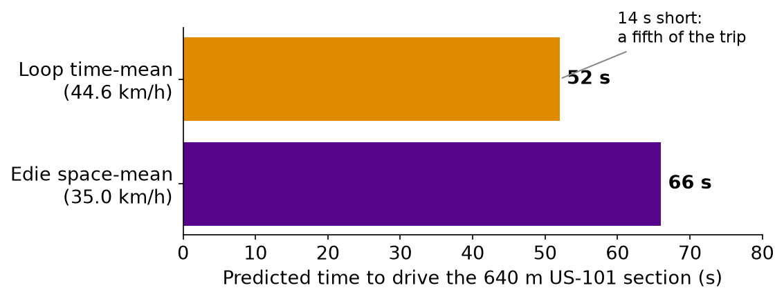
Use the loop’s number to predict travel time, and you underestimate it by about a fifth. Every travel-time sign and every navigation app faces the same choice of averages.
AI at work: from raw data to clean data
The Athens drone video with every vehicle detected and tracked by computer vision (pNEUMA Vision, EPFL, CC BY 4.0).
- Collecting: deep-learning detectors and trackers turn video into trajectories almost automatically.
- Cleaning: anomaly detection flags broken detectors: stuck at zero, frozen, or physically impossible.
- Filling gaps: imputation, from regression to neural networks, estimates missing values.
- The catch: each step is itself a model, and models can be wrong.
Part 5 · Beyond counting cars
LiDAR at the intersection
A LiDAR sensor sweeps laser pulses around itself and times each echo. Many times a second it produces a point cloud: a 3-D picture of everything in view, by day or night.
- From points to trajectories. Remove the background (road, buildings, trees), group the remaining points into objects, label each object a vehicle or a pedestrian, then follow it from frame to frame (Wu et al., TRR, 2018; Zhao et al., TR-C, 2019). The result is the trajectory of every road user: position, speed and direction.
- From the lab to the street. In 2017 Hao Xu’s group at the University of Nevada, Reno mounted a LiDAR beside Virginia Street in Reno, one of the first roadside uses of the sensor. More followed along the corridor and in Henderson, Nevada.
- Privacy by design. The data are only points: no colour, no licence plates, no faces (UNR, 2020). NCHRP’s guide to signal-based counting notes that, unlike cameras, LiDAR raises no data-privacy concerns (NCHRP Web-Only Document 436, 2025).
Watching people, not just cars
A loop detector cannot see a pedestrian, and a push button counts requests, not people. Yet pedestrians and cyclists are the road users most at risk.
- How people really cross. LiDAR at intersections in Texas and Utah tracked pedestrians and found that their crossing paths often differ from what the design assumed. The same project built a “dynamic flashing yellow arrow” that reacts to pedestrians the LiDAR sees about to cross (National Institute for Transportation and Communities, 2023).
- Seeing through a crowd. A Caltrans-funded project at UC Riverside fused camera and LiDAR data to detect pedestrians and cyclists even when they are partly hidden, with over 90% recall, and to warn connected vehicles of them (Caltrans, 2025).
Safety without waiting for crashes
Crashes are rare. Waiting for enough of them to judge an intersection can take years, and each one costs lives. Conflicts, or near misses, are far more common, and trajectories reveal them.
- Time-to-collision (TTC): how long until two road users collide if both keep their speed and path (Hayward, 1972). For a follower closing on its leader with bumper-to-bumper gap \(g\): \[ \begin{gathered} \mathrm{TTC} = \frac{g}{v_\text{follower} - v_\text{leader}}, \\ v_\text{follower} > v_\text{leader}. \end{gathered} \]
- Post-encroachment time (PET): the time between one road user leaving a conflict point and the next arriving there (Allen, Shin and Cooper, 1978).
- Measured three ways: from video (Ismail et al., TRR, 2009), from roadside LiDAR, including vehicle–pedestrian near-crashes (Wu et al., Accident Analysis & Prevention, 2018), and from simulation, with FHWA’s Surrogate Safety Assessment Model counting a conflict when TTC ≤ 1.5 s or PET ≤ 5 s by default (Gettman et al., 2008).
Road inspection: sensors on the move
Sensors do not only watch traffic. Mounted on a van driving at traffic speed, they inspect the road itself.
- Mobile LiDAR mapping. Scanners, cameras and precise positioning (GNSS and inertial sensors) map lane markings, signs, poles, manholes and bridge clearances in one pass (Guan et al., 2016). NCHRP Report 748 gives state DOTs guidelines for using it (Olsen et al., 2013).
- Pavement condition. 3-D laser systems scan a strip 4 m wide, with about 4,000 points across the lane, vertical accuracy of about ±0.5 mm and a profile every 5 mm at 100 km/h, day or night. From these scans agencies measure cracking, rutting and faulting (FHWA, 2020).
One sensor is never enough: fusion
| Sensor | Strong at | Weak at |
|---|---|---|
| Camera | detail; telling a bus from a truck from a cyclist | darkness, glare, rain, snow, fog |
| Radar | any weather, day or night; long range | coarse detail; poor at telling objects apart |
| LiDAR | precise 3-D positions; unaffected by light | cost, occlusion, heavy data; rain, snow and fog add noise |
| Loop detector | reliable counts and occupancy at one point | one point only; cannot see pedestrians |
| Phone and vehicle GPS | whole trips, citywide | only some vehicles, and not a random sample |
Sources: Yeong et al. (Sensors, 2021), Sun et al. (Sensors, 2022), NCHRP Web-Only Document 436 (2025).
Data fusion combines sensors so each covers the others’ blind spots: loops for counts plus probes for travel times, or cameras plus LiDAR for pedestrians (El Faouzi, Leung and Kurian, Information Fusion, 2011). Like the AI cleaning on the previous slide, fusion is itself a model, so it inherits the same question: how were these data made?
Part 6 · Wrap-up
Three challenges
Use the interactive figures on this page. First to share the answer with the class, with a one-line explanation, gets bragging rights.
- Sensor truce. In Build your own road, find settings where the loop and the drone agree exactly. What must be true of the traffic?
- Maximum disagreement. Make the loop report at least twice the drone’s speed. Describe the traffic you built. Where might you see it in real life?
- Truck trouble. What share of trucks makes a single loop’s speed estimate 25% too low?
Summary
- “Average speed” has two answers: time-mean (point sensors) and space-mean (snapshots, and phone pings).
- Wardrop (1952): the time-mean speed is flow-weighted, the space-mean speed is density-weighted, and \(q = k\,\bar v_s\).
- We proved \(\bar v_t = \bar v_s + \sigma_s^2/\bar v_s\), so the time-mean speed is never the smaller.
- Which average to compute depends on where the data were collected, not on which speed you want.
- Edie’s definitions work for any region, and \(q = kv\) always holds with them.
- Picking the wrong average can cost a fifth of your travel-time estimate, and a single loop can be fooled by trucks.
- Machine learning now collects, cleans and fills traffic data, but each of those steps is a model that can be wrong.
- Sensors sit in the pavement, beside the road, in vehicles or in the air, and see a point, two points, an area or a trajectory.
- LiDAR and multi-sensor systems see pedestrians, near misses and the road itself. No sensor sees everything, so agencies fuse them.
- Every sensor sees traffic through its own window. Know which window your data came from.
- Next week: the fundamental diagram, the most important curve in traffic, and the puzzles it cannot explain.
This week’s lab: Lab 1 · Real Traffic from the Sky. Build the virtual loop detector yourself, and measure the US-101 numbers above.
Notation
| Symbol | Meaning | Units |
|---|---|---|
| \(\bar v_t\) | time-mean speed: the average over vehicles passing a point | m/s or km/h |
| \(\bar v_s\) | space-mean speed: the average over vehicles on a stretch of road | m/s or km/h |
| \(\sigma_s^2\) | variance of speeds measured in space | (m/s)² |
| \(M\) | number of sub-streams in Wardrop’s model | — |
| \(q_i,\ k_i,\ v_i\) | flow, density and speed of sub-stream \(i\) | veh/h, veh/km, km/h |
| \(Q,\ K\) | total flow and total density | veh/h, veh/km |
| \(f_i,\ f_i'\) | share of sub-stream \(i\) in time (\(q_i/Q\)) and in space (\(k_i/K\)) | — |
| \(A,\ \lvert A\rvert\) | a region of the time-space diagram, and its area | —, m·s |
| \(d(A),\ t(A)\) | total distance and total time travelled by vehicles inside \(A\) | m, s |
| \(N\) | number of vehicles observed | veh |
| \(o\) | occupancy: fraction of time the loop is covered | — |
| \(d\) | loop length (not the same as Edie’s \(d(A)\)) | m |
| \(\ell,\ \ell_j\) | assumed vehicle length; length of vehicle \(j\) | m |
| \(\tau_j\) | time vehicle \(j\) covers the loop | s |
| \(T\) | length of the counting period | s |
| \(g\) | bumper-to-bumper gap between a follower and its leader | m |
| TTC | time-to-collision: time until two road users collide if neither changes speed or path | s |
| PET | post-encroachment time: time between one road user leaving a conflict point and the next arriving | s |
theme = Generators.observe(notify => {
  const read = () => notify(document.body.classList.contains("quarto-dark") ? "dark" : "light");
  read();
  const watcher = new MutationObserver(read);
  watcher.observe(document.body, {attributes: true, attributeFilter: ["class"]});
  return () => watcher.disconnect();
})
accent = theme === "dark" ? "#c9a0ff" : "#57068c"
accentRange = theme === "dark" ? ["#4b3a5c", "#ecdcff"] : ["#dccbee", "#3a0463"]
ink = theme === "dark" ? "#f2f2f2" : "black"
// Plot width: Plot's default 640 px, except on a phone, where a plot is drawn to fit its card
// instead of being shrunk (and its text with it). Changes only when the width actually changes.
plotW = Generators.observe(notify => {
  let last;
  const read = () => {
    const main = document.querySelector("main"), fit = main ? main.clientWidth - 50 : 640;
    const w = !document.querySelector(".reveal") && fit < 640 ? Math.max(240, Math.floor(fit)) : 640;
    if (w !== last) notify(last = w);
  };
  read();
  window.addEventListener("resize", read);
  return () => window.removeEventListener("resize", read);
})
⛶ Full screen · ◀ Notes · TR-GY 7353 · © 2026 Wuping Xin · CC BY-NC-SA 4.0