import sys
if "google.colab" in sys.modules:
    %pip install -q "trafficlab @ git+https://github.com/wx241/trgy7353-labs#subdirectory=sim"

import trafficlab
from trafficlab import ngsim, plotsLab 1 · Real Traffic from the Sky
NGSIM trajectories · time-space diagrams · Edie’s definitions · a virtual loop detector
 Run this lab in your browser, with nothing to install.
In 2005, the Federal Highway Administration filmed US-101 in Los Angeles from the top of a 36-storey building and turned the video into the position of every vehicle, ten times per second. In this lab you will:
- Draw a time-space diagram of real traffic, and find a stop-and-go wave in it.
- Measure flow, density and speed with Edie’s definitions (Lecture 2).
- Build a virtual loop detector, and see why it reports a different speed.
Before you start: click Open in Colab above.
1 · Load four minutes of one lane
We download lane 2 of US-101, starting at 8:00 a.m. The data arrive in feet; ngsim.load converts them to metres and seconds, and removes duplicate records, which exist in the raw data.
df = ngsim.load(location="us-101", lane=2,
                start_ms=ngsim.US101_START_MS + 600_000,   # 10 minutes after 7:50 a.m.
                seconds=240)
print(f"{len(df):,} records of {df.vehicle.nunique()} vehicles")
df.head()
77,658 records of 160 vehicles| vehicle | t | x | v | length | |
|---|---|---|---|---|---|
| 0 | 1980 | 0.0 | 637.238350 | 13.185648 | 4.1148 |
| 1 | 1980 | 0.1 | 638.551733 | 13.158216 | 4.1148 |
| 2 | 1980 | 0.2 | 639.864202 | 13.164312 | 4.1148 |
| 3 | 1980 | 0.3 | 641.182157 | 13.185648 | 4.1148 |
| 4 | 1980 | 0.4 | 642.508951 | 13.149072 | 4.1148 |
2 · The time-space diagram
Each dot is one vehicle at one instant, coloured by speed. Each vehicle leaves a streak: its trajectory.
ax = plots.time_space(df, title="US-101, lane 2, from 8:00 a.m.")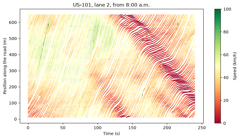
Look closely. A red band runs from the top of the road towards the bottom as time goes on. That is a stop-and-go wave, like the one on the ring road in Lecture 1.
Question 1. Read two points off the red band, and estimate the speed of the wave in km/h. Which way is it moving, compared with the traffic?
3 · Edie’s definitions
For a region A of the time-space diagram,
\begin{aligned} q(A) &= \frac{d(A)}{|A|}, \\ k(A) &= \frac{t(A)}{|A|}, \\ v(A) &= \frac{d(A)}{t(A)}, \end{aligned}
where d(A) is the total distance and t(A) the total time that vehicles spend in A.
Your turn. Complete edie below.
def edie(df, x1, x2, t1, t2, dt=0.1):
    """Flow (veh/h), density (veh/km) and speed (km/h) in the region [x1, x2] x [t1, t2].

    Each row of df is one vehicle at one instant, recorded every dt seconds.
    Hint: a row inside the region stands for dt seconds of vehicle time,
    and for v * dt metres of vehicle distance.
    """
    # YOUR CODE HERE: compute total_time t(A), total_distance d(A) and the area |A|
    return None
regions = {"A (free flow)": (300, 500, 20, 80), "B (in the wave)": (150, 350, 180, 240)}
ax = plots.time_space(df)
for name, (x1, x2, t1, t2) in regions.items():
plots.region(ax, x1, x2, t1, t2, label=name[0])
for name, box in regions.items():
result = edie(df, *box)
if result is None:
print(f"{name}: complete edie() above to see q, k and v")
else:
q, k, v = result
print(f"{name}: q = {q:5.0f} veh/h k = {k:5.1f} veh/km v = {v:5.1f} km/h "
f"(check: k*v = {k * v:5.0f})")A (free flow): complete edie() above to see q, k and v
B (in the wave): complete edie() above to see q, k and v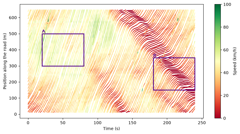
Question 2. Compare regions A and B. How do flow, density and speed change inside the wave? Does q = k\,v hold exactly? Why?
4 · A virtual loop detector
A loop detector sits at one point and records each vehicle as it passes. Your turn. Complete virtual_loop below, then compare its speeds with Edie’s space-mean speed for a region around the same point.
def virtual_loop(df, x0, t1, t2):
    """What a loop detector at position x0 would report between t1 and t2.

    Returns (count, flow in veh/h, time-mean speed in km/h, harmonic-mean speed in km/h).
    Hint: for each vehicle, find the first record at or past x0; keep it if it falls in [t1, t2).
    """
    # YOUR CODE HERE
    return None
x0, t1, t2 = 400, 0, 240
loop = virtual_loop(df, x0, t1, t2)
if loop is None:
print("Complete virtual_loop() above to see what the detector reports")
else:
n, flow, v_time, v_harm = loop
print(f"Loop at {x0} m: {n} vehicles, {flow:.0f} veh/h")
print(f" time-mean speed {v_time:5.1f} km/h")
print(f" harmonic-mean speed {v_harm:5.1f} km/h")
edie_region = edie(df, x0 - 50, x0 + 50, t1, t2)
if edie_region is not None:
print(f" Edie space-mean speed (x0 ± 50 m) {edie_region[2]:5.1f} km/h")Complete virtual_loop() above to see what the detector reportsQuestion 3. Which of the loop’s two speeds is closer to Edie’s space-mean speed? Explain why, using the rule \bar v_t = \bar v_s + \sigma_s^2/\bar v_s from Lecture 2.
Going further
- Change
laneto 1 (the leftmost lane). Is the wave there too? - Move the loop to 100 m and to 600 m. Does the reported flow change? Should it?
- The NGSIM speeds were computed from video positions, and are known to be noisy. How could you check them using
xandtalone?