1 · Why Traffic Is Weird

A jam out of nothing · trajectories · flow, density and speed

Part 1 · A jam out of nothing

The puzzle

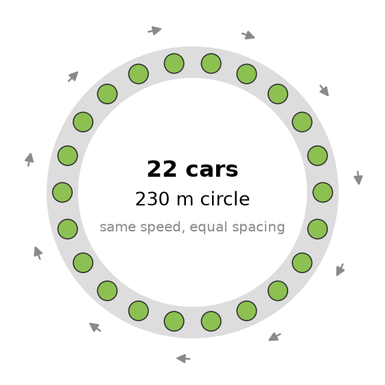
In 2008, researchers in Japan asked 22 drivers to drive around a 230 m circle, all at the same steady speed. There was no bottleneck, no accident and no traffic light. (Sugiyama et al., New Journal of Physics, 2008)

What happened next?

Before you watch: predict

Will a jam form? If one does, which way will it move: with the traffic, or against it? Make a guess before you go on.

Watch it happen

We can recreate the experiment below. Each dot is a car, coloured by its speed. The car with the black ring is you. Just wait and watch.

viewof ringN = Inputs.range([12, 30], {value: 22, step: 1, label: "Number of cars"})
viewof ringA = Inputs.range([0.2, 2.0], {value: 0.5, step: 0.1, label: "Driver responsiveness (m/s²)"})
viewof ringSpeed = Inputs.range([1, 20], {value: 8, step: 1, label: "Playback speed (× real time)"})
viewof ringRestart = Inputs.button("Restart")

// Ring road with the Intelligent Driver Model (IDM) and small random fluctuations in each driver's acceleration.
// The responsiveness and playback sliders are read live, so they can be changed without restarting.
// ringState is shared with the time-space plot, which redraws on its own timer.
ringState = { ringRestart; ringN; return {hist: [], L: 230}; }

ring = {
  const N = ringN, L = ringState.L, v0 = 12, T = 1.2, s0 = 2, b = 1.5, lc = 4, dt = 0.1, noise = 0.3;
  const x = Float64Array.from({length: N}, (_, i) => i * L / N);
  const v = new Float64Array(N).fill(6);
  const acc = new Float64Array(N);
  const hist = ringState.hist;
  const randn = () => Math.sqrt(-2 * Math.log(1 - Math.random())) * Math.cos(2 * Math.PI * Math.random());
  let t = 0, frame = 0, budget = 0, nextRecord = 0;
  while (true) {
    budget += viewof ringSpeed.value / 60;          // about 60 frames per second
    const a = viewof ringA.value;
    while (budget >= dt) {
      for (let i = 0; i < N; i++) {
        const j = (i + 1) % N;
        const gap = Math.max(((x[j] - x[i]) % L + L) % L - lc, 0.1);
        const sStar = s0 + Math.max(0, v[i] * T + v[i] * (v[i] - v[j]) / (2 * Math.sqrt(a * b)));
        acc[i] = a * (1 - (v[i] / v0) ** 4 - (sStar / gap) ** 2) + noise * randn();
      }
      for (let i = 0; i < N; i++) {
        v[i] = Math.max(0, v[i] + acc[i] * dt);
        x[i] = (x[i] + v[i] * dt) % L;
      }
      t += dt; budget -= dt;
      if (t >= nextRecord) {
        for (let i = 0; i < N; i++) hist.push({t, i, x: x[i], v: v[i]});
        nextRecord += 0.5;
        while (hist.length && hist[0].t < t - 150) hist.shift();
      }
    }
    yield {t, x: Array.from(x), v: Array.from(v), hist, frame: frame++, L};
  }
}

{
  const W = 300, R = 115;
  const color = d3.scaleSequential(d3.interpolateRdYlGn).domain([0, 8]);
  const cars = ring.x.map((xi, i) => {
    const th = 2 * Math.PI * xi / ring.L;
    return {cx: W / 2 + R * Math.cos(th), cy: W / 2 + R * Math.sin(th), fill: color(ring.v[i]), you: i === 0};
  });
  return htl.svg`<svg width="100%" viewBox="0 0 ${W} ${W}" style="max-width:${W}px;height:auto;display:block;margin:0 auto">
    <circle cx=${W / 2} cy=${W / 2} r=${R} fill="none" stroke="#ddd" stroke-width="20"/>
    ${cars.map(c => htl.svg`<circle cx=${c.cx} cy=${c.cy} r=${c.you ? 9 : 7} fill=${c.fill}
      stroke=${c.you ? ink : "#333"} stroke-width=${c.you ? 3 : 0.6} />`)}
    <text x=${W / 2} y=${W / 2 - 6} text-anchor="middle" font-size="15" fill="currentColor">t = ${ring.t.toFixed(0)} s</text>
    <text x=${W / 2} y=${W / 2 + 14} text-anchor="middle" font-size="11" fill="gray">red = slow · green = fast</text>
  </svg>`;
}

{
  const S = ringState;
  while (true) {                                    // redraw twice per second
    yield Plot.plot({
      width: plotW, height: !!document.querySelector(".reveal") ? 260 : 300,
      x: {label: "Time (s)"},
      y: {label: "Position around the ring (m)", domain: [0, S.L]},
      color: {type: "sequential", scheme: "RdYlGn", domain: [0, 8], legend: true, label: "Speed (m/s)"},
      marks: [
        Plot.dot(S.hist.slice(), {x: "t", y: "x", fill: "v", r: 1.3}),
        Plot.dot(S.hist.filter(d => d.i === 0), {x: "t", y: "x", fill: ink, r: 1.8})
      ]
    });
    await Promises.delay(500);
  }
}

Follow one driver

Keep watching the ring on the previous slide. This is your speed, the car with the black ring. Nobody ahead of you ever had a reason to stop, yet you stop and go, again and again.

{
  const S = ringState;
  while (true) {
    const mine = S.hist.filter(d => d.i === 0);
    yield Plot.plot({
      width: plotW, height: !!document.querySelector(".reveal") ? 260 : 170,
      x: {label: "Time (s)"},
      y: {label: "Your speed (m/s)", domain: [0, 9]},
      marks: [
        Plot.areaY(mine, {x: "t", y: "v", fill: accent, fillOpacity: 0.12}),
        Plot.line(mine, {x: "t", y: "v", stroke: accent, strokeWidth: 2})
      ]
    });
    await Promises.delay(500);
  }
}

The trace is live: it keeps updating while the ring runs. Stopping and starting again and again, with no bottleneck anywhere, is what a phantom jam feels like from the driver’s seat.

What just happened?

• A jam formed within minutes, exactly as in the 2008 experiment. Nobody caused it. It grew out of tiny fluctuations that each driver over-corrected.
• The red band in the right-hand plot slopes downward: the jam moves backward while every car moves forward.
• Try it: raise driver responsiveness to 1.5. The jam dissolves. Automated vehicles with well-designed cruise control could do exactly this (Lecture 9).

The plot on the right is a time-space diagram: time runs left to right and position runs bottom to top. Each car leaves a trail of dots. When the trails bunch up and turn red, cars are stopped in a jam. The jam’s boundary tilts downward because cars leave the front of the jam while new cars join its back. The jam moves backward at a speed of its own, whatever the individual cars do. By Lecture 5 you will be able to compute that speed with pencil and paper.

It happens on real freeways, every morning

This is not just a simulation. In 2005 the Federal Highway Administration filmed US-101 in Los Angeles and recorded the position of every vehicle, ten times a second. Here are four minutes of one lane:

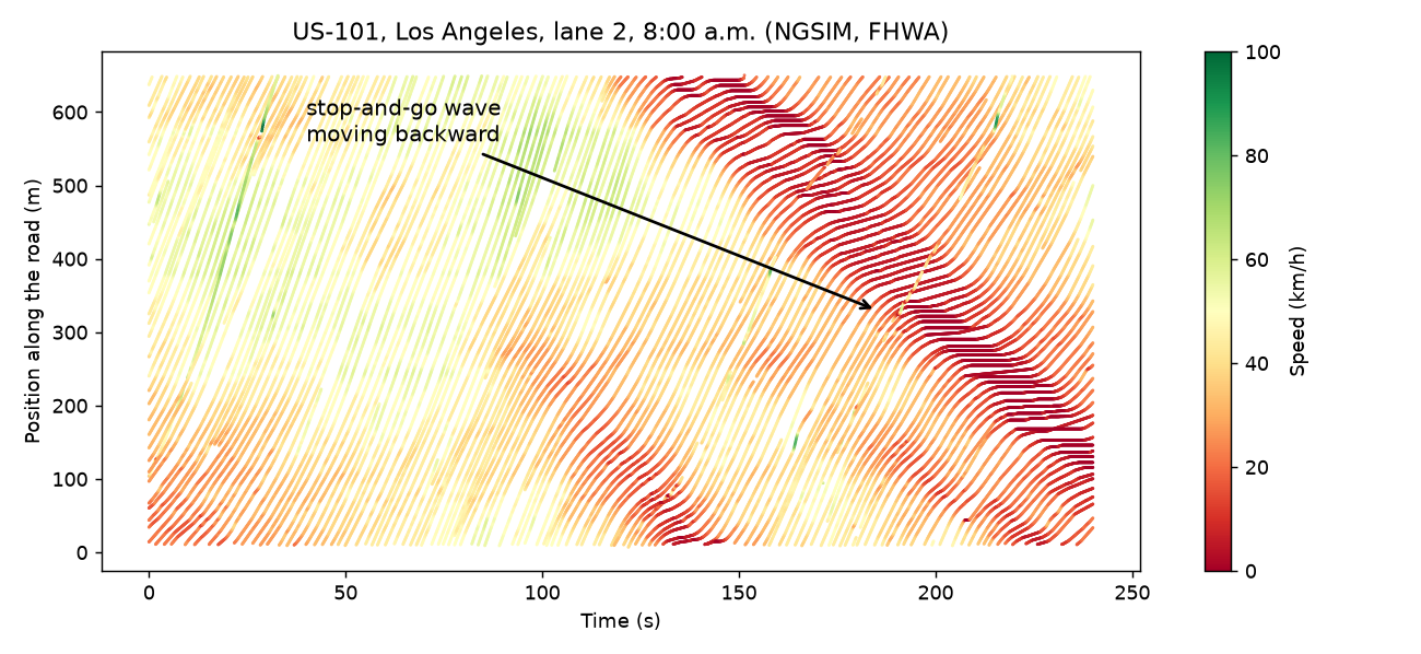
The red band is a stop-and-go wave, just like the one on the ring. It travels backward, against the traffic, at roughly 15–20 km/h. The same speed shows up on freeways all over the world. In Lab 1 you will load these data yourself and measure the wave’s speed.

The 1959 experiment: one number decides

In 1959, Robert Herman, Elliott Montroll, Renfrey Potts and Richard Rothery at General Motors Research wrote down the simplest possible driver. Each driver adjusts speed to match the car ahead, but only after a reaction time \(T\):

\[ \ddot x_{n+1}(t) = \lambda\,\big[\dot x_n(t-T) - \dot x_{n+1}(t-T)\big]. \]

Here \(\lambda\) is how strongly the driver responds. Everything depends on one number, \(C = \lambda T\): how strongly the driver reacts × how late.

Below, the leader of a line of 8 cars brakes briefly, then speeds up again. Watch what happens to the cars behind as you change \(C\).

Try it: C decides

viewof hermanC = Inputs.range([0.1, 1.8], {value: 0.75, step: 0.01, label: "C = λT (reaction strength × reaction time)"})

// Herman, Montroll, Potts and Rothery (1959): linear car-following with a delay, Euler steps of 0.01 s.
herman = {
  const N = 8, T = 1.0, dt = 0.01, tEnd = 50, lag = Math.round(T / dt), steps = Math.round(tEnd / dt);
  const lam = hermanC / T;
  const u = Array.from({length: N + 1}, () => new Float64Array(steps + 1));   // speed change of each car (m/s)
  for (let k = 1; k <= steps; k++) {
    const t = k * dt;
    u[0][k] = u[0][k - 1] + (t < 2 ? -1 : t < 4 ? 1 : 0) * dt;              // leader brakes, then recovers
    const kd = k - 1 - lag;
    for (let n = 1; n <= N; n++) {
      const a = kd >= 0 ? lam * (u[n - 1][kd] - u[n][kd]) : 0;
      u[n][k] = u[n][k - 1] + a * dt;
    }
  }
  const rows = [];
  for (let n = 0; n <= N; n++)
    for (let k = 0; k <= steps; k += 10)
      rows.push({car: n === 0 ? "Leader" : `Car ${n}`, n, t: k * dt, du: u[n][k]});
  const peak = n => u[n].reduce((m, x) => Math.max(m, Math.abs(x)), 0);
  return {rows, ratio: peak(N) / peak(1)};
}

Plot.plot({
  width: plotW, height: 320,
  x: {label: "Time (s)"},
  y: {label: "Speed change (m/s)", domain: [-6, 6], grid: true},
  color: {type: "linear", range: accentRange, domain: [-2, 8], legend: false},
  clip: true,
  marks: [
    Plot.ruleY([0]),
    Plot.line(herman.rows, {x: "t", y: "du", z: "car", stroke: "n", strokeWidth: 1.8}),
    Plot.text(herman.rows.filter(d => d.t === 0 && d.n === 0), {x: 6, y: -2.6, text: () => "Leader brakes", fill: "gray"})
  ]
})

{
  const C = hermanC, e = 1 / Math.E, h = Math.PI / 2;
  const regime =
    C <= e   ? "**Smooth and stable.** Each driver eases back to speed without overshooting, and the disturbance fades down the line."
    : C < 0.5 ? "**Oscillating, but still stable.** Drivers overshoot a little, yet the disturbance still fades from car to car."
    : C < h   ? "**Each pair is stable, but the line is not.** Every follower settles down eventually, yet the disturbance grows as it passes from car to car. On a long road, that is a phantom jam."
    :           "**Unstable.** Even a single follower overreacts more and more. In real traffic this ends in a collision."
  return md`${regime}

In this run, the last car's largest speed change is **${herman.ratio < 100 ? herman.ratio.toFixed(2) : "more than 100"} ×** the first follower's.`;
}

Stable driver, unstable line

The key idea: stability of one car is not stability of the line. Between \(C = 1/2\) and \(C = \pi/2\), every driver on their own settles down perfectly well, and yet the line of cars amplifies disturbances. That is exactly what happened on the ring road. It is also why the ring-road jam dissolved when you made drivers more attentive: faster reactions mean a smaller \(T\), and so a smaller \(C\). You will derive all three thresholds yourself in Lecture 9.

In Lab 2 you will rebuild this 1959 experiment from scratch, find the thresholds, and discover when a line of perfectly reasonable drivers crashes.

Your turn: be the smart car

The jam is back. This time you drive the black car. Tick the box, then choose one cruising speed; your car holds it smoothly, never closer to the car ahead than is safe. Can one driver dissolve the jam for all 22? Watch the jam meter.

viewof gameOn = Inputs.toggle({label: "I'm driving the black car", value: false})
viewof gameV = Inputs.range([1, 8], {value: 6, step: 0.5, label: "My cruising speed (m/s)"})
viewof gameReset = Inputs.button("Restart")

gameState = { gameReset; return {hist: [], L: 230}; }

// The ring road again. Car 0 is yours: when you drive, it holds your speed smoothly (gain 0.1 per second)
// but never accelerates more than the Intelligent Driver Model allows, so it cannot hit the car ahead.
game = {
  const S = gameState, N = 22, L = S.L, v0 = 12, T = 1.2, s0 = 2, a = 0.5, b = 1.5, lc = 4, dt = 0.1, noise = 0.3;
  const x = Float64Array.from({length: N}, (_, i) => i * L / N), v = new Float64Array(N).fill(6), acc = new Float64Array(N);
  const randn = () => Math.sqrt(-2 * Math.log(1 - Math.random())) * Math.cos(2 * Math.PI * Math.random());
  let t = 0, nextRecord = 0;
  const step = mine => {
    for (let i = 0; i < N; i++) {
      const j = (i + 1) % N, gap = Math.max(((x[j] - x[i]) % L + L) % L - lc, 0.1);
      const sStar = s0 + Math.max(0, v[i] * T + v[i] * (v[i] - v[j]) / (2 * Math.sqrt(a * b)));
      const idm = a * (1 - (v[i] / v0) ** 4 - (sStar / gap) ** 2);
      acc[i] = i === 0 && mine !== null ? Math.min(idm, 0.1 * (mine - v[i])) : idm + noise * randn();
    }
    for (let i = 0; i < N; i++) { v[i] = Math.max(0, v[i] + acc[i] * dt); x[i] = (x[i] + v[i] * dt) % L; }
    t += dt;
  };
  for (let k = 0; k < 2000; k++) step(null);            // 200 s of warm-up: the jam has formed
  const t0 = t;
  while (true) {
    const mine = viewof gameOn.value ? viewof gameV.value : null;
    for (let k = 0; k < 2; k++) step(mine);               // 12 times real time
    if (t >= nextRecord) {
      const mean = d3.mean(v), sd = d3.deviation(v);
      S.hist.push({t: t - t0, sd, mean, you: mine !== null});
      if (S.hist.length > 400) S.hist.shift();
      nextRecord = t + 1;
    }
    yield {x: Array.from(x), v: Array.from(v), L, sd: d3.deviation(v), mean: d3.mean(v)};
  }
}

{
  const W = 300, R = 115, color = d3.scaleSequential(d3.interpolateRdYlGn).domain([0, 8]);
  return htl.svg`<svg width="100%" viewBox="0 0 ${W} ${W}" style="max-width:${W}px;height:auto;display:block;margin:0 auto">
    <circle cx=${W / 2} cy=${W / 2} r=${R} fill="none" stroke="#ddd" stroke-width="20" />
    ${game.x.map((xi, i) => {
      const th = 2 * Math.PI * xi / game.L;
      return htl.svg`<circle cx=${W / 2 + R * Math.cos(th)} cy=${W / 2 + R * Math.sin(th)} r=${i === 0 ? 9 : 7}
        fill=${color(game.v[i])} stroke=${i === 0 ? ink : "#333"} stroke-width=${i === 0 ? 3 : 0.6} />`;
    })}
    <text x=${W / 2} y=${W / 2 - 4} text-anchor="middle" font-size="13" fill="gray">jam meter</text>
    <text x=${W / 2} y=${W / 2 + 22} text-anchor="middle" font-size="26" font-weight="bold"
      fill=${game.sd < 0.8 ? "#2e9e5b" : "#d7263d"}>${game.sd.toFixed(1)}</text>
  </svg>`;
}

{
  const S = gameState;
  while (true) {
    yield Plot.plot({
      width: plotW, height: 280,
      x: {label: "Time (s)"},
      y: {label: "Jam meter: spread of speeds (m/s)", domain: [0, 4], grid: true},
      marks: [
        Plot.areaY(S.hist.slice(), {x: "t", y: "sd", fill: d => d.you ? accent : "#d7263d", fillOpacity: 0.12, z: null}),
        Plot.line(S.hist.slice(), {x: "t", y: "sd", stroke: d => d.you ? accent : "#d7263d", strokeWidth: 2, z: null})
      ]
    });
    await Promises.delay(500);
  }
}

md`**Jam meter:** ${game.sd.toFixed(2)} m/s (lower is smoother) · **everyone's average speed:** ${(game.mean * 3.6).toFixed(1)} km/h · ${
  !viewof gameOn.value ? "Tick *I'm driving* to take over."
  : game.sd < 0.8 ? "**You did it.** The jam is gone, and everyone is moving faster than before."
  : "Keep trying. Hint: drive a little *slower* than feels natural, and let the gap ahead grow."}`

The winning strategy is to cruise at about 2–3 m/s. That is slower than most students choose at first. The smart car opens a gap in front of it and uses that gap to absorb each wave instead of braking. The jam meter falls from about 2.5 to 0.3, and the average speed of all 22 cars goes up, from about 7.5 to 9–10 km/h. This is the idea behind the 2017 field experiment in Tucson (Stern et al., Transportation Research Part C, 2018), where a single automated vehicle damped stop-and-go waves on a ring of about 20 cars. In Lab 12 you put one reinforcement-learning car among rule-following cars and see whether it finds a strategy like this on its own.

Part 2 · Reading traffic: trajectories

A trajectory is a story

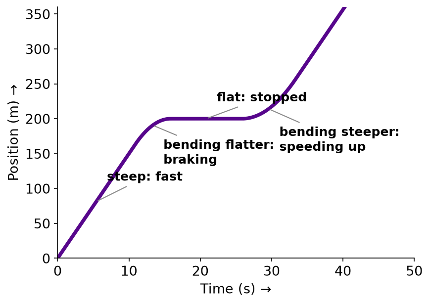
A vehicle’s trajectory is its position over time, \(x(t)\). Draw it with time across and position up, and its shape tells the story of the trip.

What you see	What it means
Slope of the line	speed, \(v = dx/dt\). Steeper is faster
Flat (horizontal) line	stopped
Bending flatter	braking
Bending steeper	speeding up

Students often want position on the horizontal axis because that is how a map looks. Insist on the convention: time runs across, position runs up. Every result in the macroscopic part of the course (waves, shocks, queues) is read off this picture.

Try it: drive one car

A car cruises, brakes for a red light at 200 m, waits, then drives off. Change how fast it goes and how long it waits, and watch the story change shape.

viewof oneV = Inputs.range([8, 25], {value: 15, step: 1, label: "Cruising speed (m/s)"})
viewof oneWait = Inputs.range([0, 30], {value: 10, step: 1, label: "Waiting at the light (s)"})

oneCar = {
  const v = oneV, dec = 3, acc = 2, stop = 200;
  const xb = stop - v * v / (2 * dec);                 // where braking starts
  const t1 = xb / v, t2 = t1 + v / dec, t3 = t2 + oneWait, t4 = t3 + v / acc;
  const pos = t => t <= t1 ? v * t
    : t <= t2 ? xb + v * (t - t1) - dec * (t - t1) ** 2 / 2
    : t <= t3 ? stop
    : t <= t4 ? stop + acc * (t - t3) ** 2 / 2
    : stop + v * v / (2 * acc) + v * (t - t4);
  const pts = d3.range(0, 70.01, 0.2).map(t => ({t, x: pos(t)})).filter(d => d.x <= 420);
  const labels = [
    {t: t1 / 2, x: pos(t1 / 2), oy: 0, text: "cruising: straight and steep"},
    {t: (t1 + t2) / 2, x: pos((t1 + t2) / 2), oy: -30, text: "braking: bends flatter"},
    {t: (t2 + t3) / 2, x: stop, oy: 28, text: "stopped: flat"},
    {t: (t3 + t4) / 2, x: pos((t3 + t4) / 2), oy: -30, text: "speeding up: bends steeper"}
  ].filter(d => d.x <= 420 && (d.text !== "stopped: flat" || oneWait > 2));
  return {pts, labels, stop};
}

Plot.plot({
  width: plotW, height: 320,
  x: {label: "Time (s)", domain: [0, 70]},
  y: {label: "Position (m)", domain: [0, 420], grid: true},
  marks: [
    Plot.ruleY([oneCar.stop], {stroke: "#d7263d", strokeDasharray: "4 3"}),
    Plot.text([{t: 69, x: oneCar.stop}], {x: "t", y: "x", text: () => "traffic light", dy: -8, textAnchor: "end", fill: "#d7263d"}),
    Plot.line(oneCar.pts, {x: "t", y: "x", stroke: accent, strokeWidth: 3}),
    Plot.dot(oneCar.labels, {x: "t", y: "x", fill: accent, r: 4}),
    Plot.link(oneCar.labels, {x1: "t", y1: "x", x2: "t", y2: d => d.x + d.oy, stroke: accent, strokeOpacity: 0.4}),
    Plot.text(oneCar.labels, {x: "t", y: d => d.x + d.oy, text: "text", dx: 6, textAnchor: "start", fontWeight: "bold"})
  ]
})

Many trajectories: the time-space diagram

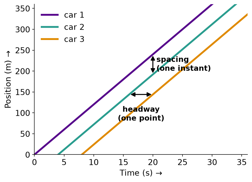
Draw every vehicle on one picture and you get a time-space diagram.

• Spacing is the vertical gap between two trajectories: how far apart two cars are at one instant.
• Headway is the horizontal gap: how much time passes between two cars at one point.
• In a single lane, trajectories never cross. A crossing means someone changed lanes, or crashed.

Spacing (m) and headway (s) are the microscopic versions of density and flow. Average spacing is 1/k, and average headway is 1/q. The next slide shows both on a live diagram.

Live: a red light and eight cars

Eight cars arrive at a traffic light, which turns red at 16 s and green at 46 s. Press Play, or drag the time slider yourself. The road is on the left; its time-space diagram is on the right. Colour shows speed: red is slow, green is fast.

viewof tsPlay = Inputs.toggle({label: "Play", value: true})
viewof tsT = Inputs.range([0, 90], {value: 0, step: 0.1, label: "Time (s)"})

// Advance the time slider while Play is on.
tsClock = {
  while (true) {
    const play = viewof tsPlay, slider = viewof tsT;
    if (play.value) {
      slider.value = slider.value >= 90 ? 0 : Math.round((slider.value + 0.2) * 10) / 10;
      slider.dispatchEvent(new Event("input", {bubbles: true}));
    }
    yield Promises.delay(40, htl.html`<span></span>`);
  }
}

// Eight cars follow the Intelligent Driver Model; during the red phase the stop line acts as a stopped vehicle.
tsSim = {
  const v0 = 15, T = 1.2, s0 = 2, a = 1.5, b = 2, lc = 5, dt = 0.1, stop = 300, red = [16, 46], n = 8;
  const enter = Array.from({length: n}, (_, i) => 3 * i);
  const x = new Array(n).fill(null), v = new Array(n).fill(v0), rows = [];
  const idm = (vi, gap, dv) => a * (1 - (vi / v0) ** 4 - ((s0 + Math.max(0, vi * T + vi * dv / (2 * Math.sqrt(a * b)))) / Math.max(gap, 0.1)) ** 2);
  for (let k = 0; k <= 900; k++) {
    const t = k * dt, isRed = t >= red[0] && t < red[1];
    for (let i = 0; i < n; i++) if (x[i] === null && t >= enter[i]) x[i] = 0;
    const acc = new Array(n).fill(0);
    for (let i = 0; i < n; i++) {
      if (x[i] === null) continue;
      let gap = Infinity, dv = 0;
      if (i > 0 && x[i - 1] !== null) { gap = x[i - 1] - x[i] - lc; dv = v[i] - v[i - 1]; }
      if (isRed && x[i] < stop && stop - x[i] - 1 < gap) { gap = stop - x[i] - 1; dv = v[i]; }
      acc[i] = Math.max(-8, gap === Infinity ? a * (1 - (v[i] / v0) ** 4) : idm(v[i], gap, dv));
    }
    for (let i = 0; i < n; i++) if (x[i] !== null) { v[i] = Math.max(0, v[i] + acc[i] * dt); x[i] += v[i] * dt; }
    if (k % 2 === 0) for (let i = 0; i < n; i++) if (x[i] !== null && x[i] <= 500) rows.push({t: +t.toFixed(1), car: i + 1, x: x[i], v: v[i]});
  }
  // headway at x = 100 m and spacing at t = 10 s, between cars 1 and 2
  const pass = (car, x0) => rows.find(r => r.car === car && r.x >= x0).t;
  const at = (car, t0) => rows.find(r => r.car === car && r.t >= t0).x;
  return {rows, stop, red, loop: 150,
          headway: {x: 100, t1: pass(1, 100), t2: pass(2, 100)},
          spacing: {t: 10, x1: at(1, 10), x2: at(2, 10)}};
}

tsNow = {
  const t = Math.round(tsT * 5) / 5;
  const cars = tsSim.rows.filter(r => Math.abs(r.t - t) < 0.05);
  const isRed = t >= tsSim.red[0] && t < tsSim.red[1];
  const passed = new Set(tsSim.rows.filter(r => r.t <= t && r.x >= tsSim.loop).map(r => r.car)).size;
  return {t, cars, isRed, passed, stopped: cars.filter(c => c.v < 0.5).length};
}

Plot.plot({
  width: plotW < 640 ? 64 : 110, height: !!document.querySelector(".reveal") ? 300 : 400, marginLeft: plotW < 640 ? 34 : 40, marginTop: 20, marginBottom: 35,
  x: {axis: null, domain: [0, 1]},
  y: {domain: [0, 500], label: "Position (m)"},
  marks: [
    Plot.rect([0], {x1: 0.25, x2: 0.75, y1: 0, y2: 500, fill: "#8883"}),
    Plot.ruleY([tsSim.stop], {x1: 0.15, x2: 0.85, stroke: tsNow.isRed ? "#d7263d" : "#2e9e5b", strokeWidth: 5}),
    Plot.rect(tsNow.cars, {x1: 0.32, x2: 0.68, y1: d => d.x - 5, y2: "x",
      fill: d => d3.interpolateRdYlGn(Math.min(d.v / 15, 1)), stroke: "#333"})
  ]
})

Plot.plot({
  width: plotW < 640 ? plotW - 64 - 24 : 640, height: !!document.querySelector(".reveal") ? 300 : 400, marginTop: 20, marginBottom: 35,
  x: {label: "Time (s)", domain: [0, 90]},
  y: {label: null, domain: [0, 500]},
  color: {type: "sequential", scheme: "RdYlGn", domain: [0, 15]},
  marks: [
    Plot.rect([0], {x1: tsSim.red[0], x2: tsSim.red[1], y1: tsSim.stop - 3, y2: tsSim.stop + 3, fill: "#d7263d"}),
    Plot.ruleY([tsSim.loop], {stroke: "#c77700", strokeDasharray: "6 4"}),
    Plot.text([0], {x: 89, y: tsSim.loop, text: () => "loop detector", dy: -7, textAnchor: "end", fill: "#c77700"}),
    Plot.line(tsSim.rows, {x: "t", y: "x", z: "car", stroke: "v", strokeWidth: 2.2}),
    Plot.arrow([tsSim.headway], {x1: "t1", x2: "t2", y1: "x", y2: "x", stroke: ink, headLength: 6, bend: false}),
    Plot.text([tsSim.headway], {x: d => (d.t1 + d.t2) / 2, y: "x", text: () => "headway", dy: 12}),
    Plot.arrow([tsSim.spacing], {x1: "t", x2: "t", y1: "x2", y2: "x1", stroke: ink, headLength: 6}),
    Plot.text([tsSim.spacing], {x: "t", y: d => (d.x1 + d.x2) / 2, text: () => "spacing", dx: -6, textAnchor: "end"}),
    Plot.ruleX([tsNow.t], {stroke: accent, strokeWidth: 2}),
    Plot.text([tsNow.t], {x: d => d, y: 490, text: () => "drone snapshot", dx: 6, textAnchor: "start", fill: accent}),
    Plot.dot(tsNow.cars, {x: "t", y: "x", r: 5, fill: ink})
  ]
})

md`**t = ${tsNow.t.toFixed(1)} s** · light is **${tsNow.isRed ? "red" : "green"}** · ${tsNow.stopped} of ${tsNow.cars.length} cars on the road are stopped · the loop detector has counted **${tsNow.passed}** cars · the drone sees **${tsNow.cars.length}**`

Point out the two lines drawn on the diagram. The loop detector is a horizontal line: one position, all times. The drone snapshot is a vertical line: one instant, all positions. A GPS probe would be a single trajectory. Every sensor sees the diagram through its own slice, and Lecture 2 builds on exactly this.

Can you read it?

Use the red-light diagram on the previous slide.

1. While the light is red, the points where trajectories turn flat move down the diagram, one car after another. What is moving down, and roughly how fast?
2. When the light turns green, the cars do not all start together. Where does the “start moving” signal travel?
3. The stopped cars have the smallest spacing of all, yet during the red no car passes the stop line. So is a queue “high density, zero flow”? Where is the flow highest just after the green?

Answers

1. The back of the queue. It moves upstream, against the traffic, as each arriving car stops a little further back. Its speed is the slope of the line joining the points where the trajectories turn flat. This is a shock wave, the subject of Lecture 5.
2. Backward, from the stop line upstream. Each car can start only after the car ahead has moved. This start-up wave travels upstream at roughly 15–20 km/h, like the waves on the ring road and on US-101.
3. Yes: the queue is at jam density with zero flow. Just after the green, flow is highest at the stop line, where cars leave the queue at the road’s capacity. That is exactly the point where a traffic engineer would measure saturation flow.

Trajectories at work: traffic signals

The red-light diagram you just read is exactly how engineers now evaluate real signals, using trajectories from connected vehicles and phones instead of detectors in the pavement.

• Retiming signals with a few percent of cars. Henry Liu’s group at Michigan retimed 34 signals in Birmingham, Michigan using only GM vehicle trajectories, about 7% of traffic. Delay fell by up to about 20% and stops by up to about 30% (Wang et al., Nature Communications, 2024). Earlier, with DiDi, the same group optimized signals in Jinan, China from ride-hailing trajectories (Zheng et al., TRB, 2018).
• Signal report cards. Purdue’s group (Darcy Bullock) computes arrivals on green, split failures and level of service from commercial connected-vehicle data, with no detectors at all (Saldivar-Carranza et al., TRR, 2021), including diamond and diverging diamond interchanges (J. Transportation Technologies, 2021 and 2022).
• Coordinating an arterial. Jianyuan Xu and Zong Tian at the University of Nevada, Reno use trajectories to evaluate arterial coordination (Xu et al., IJTST, 2025) and to split a corridor into coordinated groups by where drivers actually go (Xu and Tian, TRR, 2023).

More in Lecture 5 (queues and shock waves) and Lecture 12 (a real signal controller in the loop).

The key idea: no single connected vehicle tells you much, but thousands of them, overlaid on one time-space diagram for the same intersection and the same time of day, reveal the queue, the arrivals on green and the delay. That is the red-light diagram on the previous slides, filled in with real data. Purdue calls its version the “Purdue Probe Diagram”.

Trajectories at work: automated vehicles

• Learning how people drive. Car-following and lane-changing models are calibrated on trajectories. Deep learning can go further: Zhu, Wang and Wang (TR-C, 2018) trained a human-like car-following model on 2,000 events from the Shanghai Naturalistic Driving Study.
• Testing automated vehicles. Dangerous situations are rare in real driving, so testing on public roads alone would take enormous mileage. Feng et al. (Nature, 2023) trained background vehicles on naturalistic driving data, then edited their behavior to keep only the safety-critical moments, making tests far faster while staying statistically unbiased.
• Naturalistic driving data follow one driver for months, instead of every vehicle on one stretch of road. The largest, the SHRP2 study (2010–2013), instrumented the cars of more than 3,400 US drivers: about 5.4 million trips and over 1,500 crashes on video.

More in Lecture 8 (car-following), Lecture 9 (automated vehicles and phantom jams), Lecture 10 (calibration) and Lecture 12 (reinforcement learning).

Trajectories beyond this course: travel demand

Can trajectories feed travel demand models? Yes, but not the ones in Lab 1.

	High-frequency trajectories	Sparse GPS traces
Examples	NGSIM, highD	phones, ride-hailing, connected vehicles
Sampling	10–25 times a second	every few seconds to minutes
Coverage	every vehicle, a few hundred metres	some vehicles, the whole city, whole trips
Good for	traffic flow, driver behavior	origins and destinations, route choice

Sparse traces are now a major input to demand models: origin–destination matrices from phone location data (Çolak et al., TRR, 2015) and route choice from smartphone GPS (Bierlaire, Chen and Newman, TR-C, 2013). The catch: only some travelers are observed, and not a random sample, so the data must be expanded and corrected for bias.

Where do trajectories come from?

Dataset	Where	How	What
NGSIM (FHWA, 2005–06)	US-101 and Lankershim Blvd (Los Angeles), I-80 (Emeryville, CA), Peachtree St (Atlanta)	video from tall buildings, 10 Hz	every vehicle, about 500–700 m
highD (RWTH Aachen, 2017–18)	German highways near Cologne	drone video, 25 Hz	110,000 vehicles, 16.5 h
inD, rounD, exiD	German intersections, roundabouts, ramps	drone video	cars, trucks, cyclists, pedestrians
pNEUMA (EPFL, 2018)	central Athens	a swarm of 10 drones	almost half a million trajectories
I-24 MOTION (Vanderbilt)	4.2 miles of I-24, Nashville	276 pole-mounted cameras	every vehicle, every morning
TGSIM (FHWA)	Chicago, Washington DC	helicopters and fixed cameras	human drivers next to automated vehicles
Waymo Open Motion, Argoverse 2	US cities	sensors on self-driving cars	the scene around one vehicle

Full trajectories of every vehicle are rare and precious. Most traffic data are only slices of the time-space diagram, such as a line at one point or a snapshot at one instant. What each slice can and cannot tell us is Lecture 2. In Lab 1 you will load real NGSIM trajectories yourself.

NGSIM: why the data had to be rebuilt

NGSIM turned video into trajectories automatically. Positions were close, but speeds and accelerations come from differentiating positions, and differentiating amplifies every small error.

• Raw NGSIM contains large measurement errors (Punzo, Borzacchiello and Ciuffo, TR-C, 2011): accelerations no car can produce, speeds that jump in steps, and followers that drive through their leader (Coifman and Li, TR-B, 2017).
• Smoothing: filter the positions before differentiating (Thiemann, Treiber and Kesting, TRR, 2008).
• Reconstruction: Montanino and Punzo (TR-B, 2015) rebuilt the I-80 data so every trajectory obeys physics and every leader–follower pair stays consistent. With the rebuilt data, models reproduced the observed jams better.
• Re-extraction: Coifman and Li (TR-B, 2017) went back to the original video and re-tracked vehicles by hand. They argued that some errors cannot be cleaned away, and they found 11% more vehicles.

The lesson: calibrate a car-following model on raw NGSIM and it learns the noise, not the driver. Always check a trajectory’s speed and acceleration before trusting it. You will see this in Lab 1, and it matters again in Lectures 8 and 10.

Ask students: if position is accurate to half a metre, and samples are 0.1 s apart, how large an error in speed can one bad sample create? Half a metre over 0.1 s is 5 m/s, or 18 km/h. Differentiate again for acceleration and the error is 50 m/s², five times gravity. That is why raw accelerations look absurd.

Part 3 · Three numbers describe traffic

Flow, density and speed

Variable	Symbol	Units	Measures
Flow	\(q\)	veh/h	vehicles passing a point per hour
Density	\(k\)	veh/km	vehicles on a stretch of road
Speed	\(v\)	km/h	how fast they move

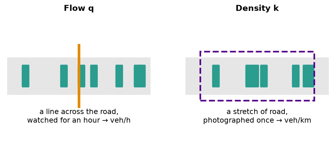
In a steady stream they are linked by

\[ q = k\,v. \]

Check it on the ring: 22 cars on 230 m is a density of about 96 veh/km. If they all drive at 6 m/s (21.6 km/h), the flow past any point is \(q = 96 \times 21.6 \approx 2070\) veh/h.

Try it: the fundamental diagram

Greenshields (1935) proposed that speed falls linearly as density rises: \(v = v_f\,(1 - k/k_j)\). Then \(q = v_f\,k\,(1 - k/k_j)\). Move the sliders and watch the road’s capacity change.

viewof vf = Inputs.range([60, 130], {value: 100, step: 1, label: "Free-flow speed vf (km/h)"})
viewof kj = Inputs.range([80, 200], {value: 150, step: 1, label: "Jam density kj (veh/km)"})

Plot.plot({
  width: plotW, height: 300,
  x: {label: "Density k (veh/km)", domain: [0, 200]},
  y: {label: "Flow q (veh/h)", domain: [0, 6500], grid: true},
  marks: [
    Plot.line(d3.range(0, kj + 0.01, kj / 200).map(k => ({k, q: vf * k * (1 - k / kj)})),
              {x: "k", y: "q", stroke: accent, strokeWidth: 3}),
    Plot.dot([{k: kj / 2, q: vf * kj / 4}], {x: "k", y: "q", r: 6, fill: accent}),
    Plot.ruleY([0])
  ]
})

md`**Capacity:** ${Math.round(vf * kj / 4)} veh/h at critical density ${kj / 2} veh/km.`

Part 4 · Wrap-up

This semester, you will learn to…

• Explain where jams come from, how fast they move, and when they clear (Lectures 3–6)
• Build your own traffic simulator in Python, piece by piece (all semester)
• Measure traffic from real data: drone and roadside video, freeway sensors (Lectures 1–4)
• Fit models to data, and know how much to trust them (Lecture 10)
• Use AI well: estimating and forecasting traffic, reinforcement learning, and knowing when a simple rule wins (Lectures 9, 11 and 12)
• Understand digital twins: simulations kept in sync with real roads, with real signal controllers plugged in (Lecture 12)

Three challenges

Use the simulations on this page. First to share the answer with the class, with a one-line explanation, gets bragging rights.

1. Fewest cars. With driver responsiveness at 0.5, what is the smallest number of cars on the ring that still produces a jam? Why does a jam need enough cars?
2. Just attentive enough. With 22 cars, what is the lowest driver responsiveness that keeps traffic smooth?
3. The tipping point. In the 1959 experiment, find the value of \(C\) at which the last car’s disturbance is exactly as large as the first follower’s. Theory says \(1/2\). Do you get \(1/2\)? (Lab 2 explains why not.)

Summary

• Jams can appear out of nothing, and they travel backward.
• A driver who is stable alone can still be part of an unstable line of cars: \(C = \lambda T\) decides.
• Trajectories and the time-space diagram contain all the information about a traffic stream.
• Flow, density and speed summarize it, and \(q = kv\) links them.
• Next week: what sensors really measure, and why “average speed” has two different answers.

This week’s labs: Lab 1 · Real Traffic from the Sky and Lab 2 · Phantom Jams on Your Laptop. Both run in Colab with one click.

Play more: the Shock Wave Builder previews Lecture 5.

Notation

Symbol	Meaning	Units
\(t\)	time	s
\(x(t)\)	position of a vehicle along the road: its trajectory	m
\(v = dx/dt\)	speed	m/s or km/h
\(a = d^2x/dt^2\)	acceleration	m/s²
\(s,\ h\)	spacing (distance to the car ahead), headway (time to the car ahead)	m, s
\(q\)	flow: vehicles passing a point per unit time	veh/h
\(k\)	density: vehicles per unit length of road	veh/km
\(v_f,\ k_j\)	free-flow speed, jam density	km/h, veh/km
\(k_c,\ q_{\max}\)	critical density, capacity (the top of the fundamental diagram)	veh/km, veh/h
\(T\)	driver reaction time (Herman et al.)	s
\(\lambda\)	driver sensitivity: how strongly a driver responds	1/s
\(C = \lambda T\)	the one number that decides stability	—

theme = Generators.observe(notify => {
  const read = () => notify(document.body.classList.contains("quarto-dark") ? "dark" : "light");
  read();
  const watcher = new MutationObserver(read);
  watcher.observe(document.body, {attributes: true, attributeFilter: ["class"]});
  return () => watcher.disconnect();
})
accent = theme === "dark" ? "#c9a0ff" : "#57068c"
accentRange = theme === "dark" ? ["#4b3a5c", "#ecdcff"] : ["#dccbee", "#3a0463"]
ink = theme === "dark" ? "#f2f2f2" : "black"
// Plot width: Plot's default 640 px, except on a phone, where a plot is drawn to fit its card
// instead of being shrunk (and its text with it). Changes only when the width actually changes.
plotW = Generators.observe(notify => {
  let last;
  const read = () => {
    const main = document.querySelector("main"), fit = main ? main.clientWidth - 50 : 640;
    const w = !document.querySelector(".reveal") && fit < 640 ? Math.max(240, Math.floor(fit)) : 640;
    if (w !== last) notify(last = w);
  };
  read();
  window.addEventListener("resize", read);
  return () => window.removeEventListener("resize", read);
})